Kähler manifolds and groups, part 1

One of the nice things about living in Hyde Park is the proximity to the University of Chicago. Consequently, over the summer I came in to the department from time to time to work in my office, where I have all my math books, fast internet connection, etc. One day in early September (note: the Chicago quarter doesn’t start until October, so technically this was still “summer”) I happened to run in to Volodya Drinfeld in the hall, and he asked me what I knew about fundamental groups of (complex) projective varieties. I answered that I knew very little, but that what I did know (by hearsay) was that the most significant known restrictions on fundamental groups of projective varieties arise simply from the fact that such manifolds admit a Kähler structure, and that as far as anyone knows, the class of fundamental groups of projective varieties, and of Kähler manifolds, is the same.

Based on this brief interaction, Volodya asked me to give a talk on the subject in the Geometric Langlands seminar. On the face of it, this was a ridiculous request, in a department that contains Kevin Corlette and Madhav Nori, both of whom are world experts on the subject of fundamental groups of Kähler manifolds. But I agreed to the request, on the basis that I (at least!) would get a lot out of preparing for the talk, even if nobody else did.

Anyway, I ended up giving two talks for a total of about 5 hours in the seminar in successive weeks, and in the course of preparing for these talks I learned a lot about fundamental groups of Kähler manifolds. Most of the standard accounts of this material are aimed at people whose background is quite far from mine; so I thought it would be useful to describe, in a leisurely fashion, and in terms that I find more comfortable, some elements of this theory over the course of a few blog posts, starting with this one.

This post is a gentle introduction to the (mostly local) geometry of Kähler manifolds themselves. Everything I say here is completely standard, and can be found in all the standard references (e.g. Griffiths and Harris; another very nice reference is Lectures on Kähler geometry by Moroianu). The main reason to go through this material so explicitly is to make transparent what parts of the theory still hold, and what need to be modified, when one considers the geometry of noncompact Kähler manifolds, especially those arising as (infinite) covering spaces of compact ones; but this point will need to wait to a subsequent post to be validated. The definition of a Kähler manifold has two parts: a linear algebra condition, and an integrability condition. We discuss these in turn.

1. Linear algebra

A Euclidean structure on V is just a positive definite symmetric inner product. After a change of basis, we can identify V with $\mathbb{R}^{2n}$ with its “standard” inner product (i.e. dot product). Thus the group of linear transformations of V preserving a positive definite symmetric inner product is isomorphic to the orthogonal group $\text{O}(2n,\mathbb{R})$ .

A complex structure on V is just a linear endomorphism J which squares to -1. Since V is real, the eigenvalues of J are i and -i, each occurring with multiplicity equal to half the dimension of V (so the dimension of V had better be even). The endomorphism J extends by linearity to a complex-linear endomorphism of the complexification $V_{\mathbb{C}}:=V \otimes \mathbb{C}$ , where it becomes diagonalizable, and there is a canonical decomposition $V_{\mathbb{C}}=V' \oplus V''$ where V’ is the i-eigenspace, and V” is the -i-eigenspace of J. For any vector v in V there is a canonical decomposition

$v = \frac 1 2 (v - iJv) + \frac 1 2 (v+iJv)$

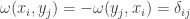
which we write as v = v’ + v”, where v’ is in V’ and v” in V”. The map from V to V’ taking v to v’ takes the operator J to multiplication by i, and identifies V with the complex vector space V’. Thus the group of (real) linear transformations of V preserving J is isomorphic to the complex linear group $\text{GL}(n,\mathbb{C})$ .

A symplectic structure on V is a non-degenerate antisymmetric inner product. This means a bilinear map $\omega:V \times V \to \mathbb{R}$ satisfying $\omega(v,w) = -\omega(w,v)$ , and such that for any nonzero v there is a nonzero w with $\omega(v,w)\ne 0$ . After a change of basis, we can identify V with $\mathbb{R}^{2n}$ with its “standard” symplectic product; i.e. if we choose basis vectors $x_1,\cdots,x_n,y_1,\cdots,y_n$ then

$\omega(x_i,y_j) = -\omega(y_j,x_i) = \delta_{ij}$ , and $\omega(x_i,x_j) = \omega(y_i,y_j) = 0$

Thus the group of linear transformations of V preserving a symplectic form is isomorphic to the symplectic group $\text{Sp}(2n,\mathbb{R})$ .

Thus, a real vector space V of even dimension can admit a Euclidean structure, a complex structure, and a symplectic structure. These three structures are said to be compatible if they satisfy

$\langle v,w\rangle = \langle Jv,Jw\rangle, \quad \omega(v,w) = \langle Jv,w\rangle, \quad \omega(v,w) = \omega(Jv,Jw)$

for any two vectors v and w. Note that any two of these conditions implies the third. At the level of Lie groups, compatibility can be expressed in terms of the intersection of the stabilizers of the three structures:

$\text{Sp}(2n,\mathbb{R}) \cap \text{O}(2n,\mathbb{R}) = \text{U}(n)$ ,
$\text{Sp}(2n,\mathbb{R}) \cap \text{GL}(n,\mathbb{C}) = \text{U}(n)$ , and
$\text{O}(2n,\mathbb{R}) \cap \text{GL}(n,\mathbb{C}) = \text{U}(n)$

Thus any two of the three structures (Euclidean, complex, symplectic) are compatible if the intersections of their stabilizers are isomorphic to a copy of the unitary group. The unitary group is the group of complex linear automorphisms of a complex vector space preserving a Hermitian form. This arises in the following way: a symmetric definite inner product on V induces a symmetric complex bilinear pairing on $V_{\mathbb{C}}$ , and thereby a sesquilinear pairing H defined by

$H(v,w) = \langle v,\overline{w}\rangle_{\mathbb{C}}$

The restriction of H defines a Hermitian pairing on V’; identifying V’ with V gives a complex valued (real!) linear pairing on V whose real part is the given inner product, and whose imaginary part is the given symplectic form.

2. Integrability, and Kähler manifolds

Now let M be a real 2n-dimensional manifold. A Riemannian metric on M is a smoothly varying choice of positive definite inner product on the tangent spaces to M at each point. An almost complex structure is a smoothly varying choice of complex structure on the tangent spaces to M at each point. An almost symplectic structure is a smoothly varying choice of symplectic structure on the tangent spaces to M at each point. Expressed in terms of tensors, the Riemannian metric is a symmetric 2-form g, the almost complex structure is a section J of $\text{End}(T M)$ squaring to -1 pointwise, and the almost symplectic structure is an alternating 2-form $\omega$ .

The field of endomorphisms J determines a splitting of the complexification of T M into T’M and T”M pointwise. An almost complex structure is integrable if the bundle T’M is integrable; i.e. if the Lie bracket of two sections of this bundle is also a section of this bundle. Such a structure gives M the structure of a complex manifold, and is equivalent to the existence of an atlas of charts modeled on $\mathbb{C}^n$ for which the transition functions between charts are holomorphic. An almost symplectic structure is integrable if the 2-form $\omega$ is closed; i.e. if $d\omega = 0$ as a form. Such a structure gives M the structure of a symplectic manifold, and is equivalent to the existence of an atlas of charts modeled on $\mathbb{R}^{2n}$ for which the transition functions between charts are symplectomorphisms (i.e. the derivative of the transition function at every point is a symplectic matrix).

Definition: A real 2n-manifold is Kähler if it admits a Riemannian metric, a complex structure, and a symplectic structure which are compatible at every point.

Every smooth manifold admits a Riemannian metric, and a manifold admits an almost complex structure if and only if it admits an almost symplectic structure (and either condition can be expressed in terms of properties of the characteristic classes of the tangent bundle). But the condition of integrability is much more subtle (at least for closed manifolds; any almost symplectic structure on an open manifold is homotopic to an integrable one).

Definition: A finitely presented group G is a Kähler group if it is equal to the fundamental group of a closed (i.e. compact without boundary) Kähler manifold.

Note that since the Kähler condition is preserved under taking covers and products, the class of Kähler groups is closed under passing to finite index subgroups, and taking (finite) products.

On any complex manifold we can choose coordinates locally $x_1,\cdots,x_n,y_1,\cdots,y_n$ so that the vector fields

$\partial_{z_j}:=\frac 1 2 (\partial_{x_j} - i \partial_{y_j})$

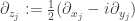
are sections of T’M. The dual 1-forms $dz_j: = dx_j + i dy_j$ and $d\overline{z}_j:=dx_j - i dy_j$ are a local basis for the smooth complex-valued 1-forms $\Omega^1_{\mathbb{C}}$ , and any complex 2-form can be expressed locally in the form

$h: = \sum h_{\alpha\overline{\beta}} dz_{\alpha} \otimes d\overline{z}_{\beta}$

A Hermitian metric H determines such an h by $H(v,w) = h(v,\overline{w})$ ; the Hermitian condition is equivalent to the symmetry of h (i.e. that $h_{\alpha\overline{\beta}} = \overline{h_{\beta\overline{\alpha}}}$ ) and positivity (i.e. that $h(v,\overline{v})$ is real and positive for all nonzero v). Any Riemannian metric on a complex manifold can be averaged under the action of J pointwise and then complexified and restricted to T’M to produce a Hermitian metric. Taking imaginary parts gives rise to an alternating 2-form

$\omega:=\frac i 2 \sum h_{\alpha\overline{\beta}} dz_\alpha\wedge d\overline{z}_\beta$

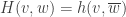
which is nondegenerate pointwise (i.e. $\omega^n$ is nowhere zero). The metric is Kähler if and only if $d\omega=0$ .

Now, on a Riemannian manifold, one may always locally choose geodesic normal coordinates, centered at any given point, and in which the metric tensor g osculates the Euclidean metric (in these coordinates) to first order; i.e.

$g_{ij} = \delta_{ij} + O(2)$

where O(2) denotes terms vanishing to at least 2nd order at the center. One way to find such coordinates is to take Euclidean coordinates on the tangent space at the center point, and push them forward by the exponential map. For a Hermitian metric on a complex manifold, one can choose holomorphic local coordinates with this property if and only if the metric is Kähler; that is,

Proposition: A Hemitian metric h on a complex manifold M is Kähler if and only if there are local holomorphic coordinates at any point for which

$h_{\alpha\overline{\beta}} = \delta_{\alpha\beta} + O(2)$

One direction of this proposition is easy: for such a choice of coordinates, the form $\omega$ is constant up to first order, and therefore $d\omega=0$ at the given point. But the definition of exterior d is coordinate free, and therefore $d\omega=0$ holds everywhere.

3. Dolbeault Cohomology

On any almost complex manifold M, the decomposition of the complexified tangent space into T’ and T” gives rise to a decomposition of its dual space, and we can decompose the space of complex-valued n-forms $\Omega^n_{\mathbb{C}}$ into components $\oplus_{p+q=n} \Omega^{p,q}$ One coordinate-free way to see this decomposition is to extend the action of J on the (complexified) tangent space to an action of the circle (by complex linearity); this gives rise to an action of the circle on the complexified cotangent spaces, and to all its tensor powers. Thus the space of complex-valued n-forms decomposes into invariant subspaces for this circle action; the fiber of $\Omega^{p,q}$ over each point is the subspace where $e^{i\theta}$ acts as multiplication by $e^{i(p-q)\theta}$ .

If the almost complex structure is integrable, we can choose holomorphic coordinates $z_j$ locally, and then $\Omega^{p,q}$ is spanned by forms

$dz_{i_1}\wedge \cdots \wedge dz_{i_p} \wedge d\overline{z}_{j_1}\wedge \cdots \wedge d\overline{z}_{j_q}$

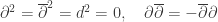
Thus (by differentiating in the usual way) we see that $d\Omega^{p,q} \subset \Omega^{p+1,q}\oplus \Omega^{p,q+1}$ (this fact is equivalent to the integrability of the complex structure) and we can decompose d into $\partial$ and $\overline{\partial}$ respectively, where $\partial \Omega^{p,q} \subset \Omega^{p+1,q}$ and $\overline{\partial} \Omega^{p,q} \subset \Omega^{p,q+1}$ . These operators satisfy

$\partial^2 = \overline{\partial}^2 = d^2 = 0, \quad \partial \overline{\partial} = -\overline{\partial} \partial$

So, for example, on a Kähler manifold, the symplectic form $\omega$ is both real (i.e. contained in ordinary $\Omega^2$ ) and of type $\Omega^{1,1}$ in $\Omega^2_{\mathbb{C}}$ .

Since $\overline{\partial}^2=0$ , the various $\Omega^{p,*}$ form a complex, whose homology groups are the Dolbeault cohomology, denoted $H^{p,q}_{\overline{\partial}}$ . By analogy with the Poincaré lemma (which proves vanishing of ordinary de Rham cohomology of smooth manifolds locally) there is the Dolbeault Lemma, which says that any form $\alpha$ with $\overline{\partial}\alpha = 0$ can be locally written as $\alpha = \overline{\partial}\beta$ . This lets us take resolutions and compute cohomology; if we write $\Omega^p_h$ for the sheaf of holomorphic p-forms (i.e. those $\Omega^{p,0}$ forms which are in the kernel of $\overline{\partial}$ ) then we obtain the

Dolbeault Theorem: for any complex manifold M, there is an isomorphism $H^q(M,\Omega^p_h) = H^{p,q}_{\overline{\partial}}(M)$ .

In particular, $H^{p,0}_{\overline{\partial}}(M)$ can be identified with the global holomorphic p-forms, which we denote (by abuse of notation) also by $\Omega^p_h$ .

From the Dolbeault Lemma one can also deduce the following:

Local $i\partial\overline{\partial}$ Lemma: if $\omega$ is a real 2-form of type $\Omega^{1,1}$ , then $d\omega=0$ if and only if we can write $\omega$ locally in the form $i\partial\overline{\partial} u$ for some real function $u$ .

If $\omega$ is exact, such a function u can be found globally. When M is Kähler, the symplectic form $\omega$ can be expressed locally in the form $i\partial\overline{\partial} u$ ; such a function u is called a (local) Kähler potential. Conversely, every local potential u on a complex manifold for which the form $i\partial\overline{\partial} u$ is nondegenerate (i.e. satisfies $\omega^n \ne 0$ in its domain of definition) gives the manifold locally the structure of a Kähler manifold. Note that a Kähler potential cannot exist globally on a compact Kähler manifold.

4. Hodge theory

A Riemannian metric on a manifold induces inner products on the fibers of all natural bundles over the manifold, including the cotangent bundle and its tensor and exterior powers. On a Riemannian manifold of dimension n there is a Hodge star $*:\Omega^k \to \Omega^{n-k}$ defined pointwise by

$\alpha \wedge *\beta = \langle \alpha,\beta\rangle d\text{vol}$

and we get an inner product on forms by $(\alpha,\beta) = \int_M \alpha \wedge *\beta$ .

The Hodge star operator satisfies the identity $*^2 = -1^{k(n-k)}$ on k-forms. Define an operator $\delta:=-(-1)^{nk}*d*$ from $\Omega^k$ to $\Omega^{k-1}$ for each k, and define the Laplacian to be the operator $\Delta:=d\delta + \delta d$ .

A form $\alpha$ is harmonic if $\Delta \alpha = 0$ ; the harmonic p-forms are denoted $\mathcal{H}^p$ . On any compact manifold there is a Hodge decomposition

$\Omega^p = \mathcal{H}^p \oplus d\Omega^{p-1} \oplus \delta \Omega^{p+1}$

where the summands are orthogonal. One deduces that there is an isomorphism $H^p = \mathcal{H}^p$ , and that every (de Rham) cohomology class contains a unique harmonic representative, which is also the unique representative of smallest norm.

Again on a compact manifold, it turns out that $\delta$ is the formal adjoint of d with respect to the pairing on p-forms (for any p), and therefore that

$(\Delta \alpha,\alpha) = (d\alpha,d\alpha) + (\delta \alpha,\delta\alpha)$

One proves this by integration by parts, since the difference between the two sides differs by the integral of an exact form. Thus, a form is harmonic if and only if it is closed and coclosed (i.e. in the kernel of $\delta$ ).

On a complex manifold we extend Hodge star to complex-valued forms so that $\alpha \wedge *\overline{\beta} = \langle \alpha,\beta\rangle d\text{vol}$ is the local Hermitian pairing. Thus $*:\Omega^{p,q} \to \Omega^{n-q,n-p}$ . We can define formal adjoints

$\partial^*:=-*\overline{\partial}*, \quad \overline{\partial}^*: = -*\partial *$

and Laplace operators

$\Delta_\partial:=\partial\partial^* + \partial^*\partial, \quad \Delta_{\overline{\partial}}:=\overline{\partial}\overline{\partial}^* + \overline{\partial}^*\overline{\partial}$

On a Kähler manifold, a surprisingly difficult local calculation gives the crucial identity

$\Delta = 2\Delta_{\partial} = 2\Delta_{\overline{\partial}}$

and therefore the (p,q) components of a harmonic p+q form are themselves harmonic!

Explicitly, we have a Hodge decomposition for (p,q)-forms using $\Delta_{\overline{\partial}}$ :

$\Omega^{p,q} = \mathcal{H}^{p,q} \oplus \overline{\partial} \Omega^{p,q-1} \oplus \overline{\partial}^* \Omega^{p,q+1}$

where $\mathcal{H}^{p,q}$ are the (p,q)-forms in the kernel of $\Delta_{\overline{\partial}}$ , from which one deduces the Dolbeault isomorphism $H^{p,q}_{\overline{\partial}} = \mathcal{H}^{p,q}$ ; but from $\Delta = 2\Delta_{\overline{\partial}}$ one also gets the decomposition

$\mathcal{H}^k = \oplus_{p+q=k} \mathcal{H}^{p,q}$

One immediate miracle is the fact that on a Kähler manifold, holomorphic forms are harmonic. Explicitly, a (p,q)-form $\alpha$ on a compact manifold is harmonic if and only if $\overline{\partial} \alpha = 0$ and $\overline{\partial} ^*\alpha = 0$ . This follows from the identity

$(\Delta_{\overline{\partial}} \alpha,\alpha) = (\overline{\partial}\alpha,\overline{\partial}\alpha) + (\overline{\partial}^* \alpha,\overline{\partial}^*\alpha)$

proved as before by integrating by parts. But for a (p,0) form, the operator $\overline{\partial}^*$ is identically zero (since its image is in $\Omega^{p,-1} = 0$ ), and a (p,0) form is in the kernel of $\overline{\partial}$ if and only if it is holomorphic.

One reason to be impressed by this miracle is that the condition of being harmonic depends very delicately on the choice of a Riemannian metric, whereas the condition of being holomorphic depends only on the complex structure. Usually, the harmonic forms are only as regular as the metric; a Kähler metric is typically only smooth (one sees this by starting with one Kähler form and perturbing it by adding something of the form $i\partial\overline{\partial} u$ for u a small bump function) whereas a complex structure is analytic. Anyway, this miracle has another miraculous consequence: since the wedge product of two holomorphic forms is holomorphic, it follows that the wedge product of two harmonic forms of type (p,0) and (q,0) is also harmonic, of type (p+q,0). As a rule of thumb, wedge products of harmonic forms (even on a Kähler manifold) is almost never harmonic, so this is an extraordinary fact.

Example: Let S be a closed Riemann surface of genus at least 2. There is a natural complex structure on S, and any Riemannian metric can be averaged under J to define a Hermitian metric, whose associated 2-form is automatically closed because S is 2-dimensional (as a real manifold). So S is Kähler. Let $\alpha$ and $\beta$ be two real harmonic 1-forms which are not proportional; for instance, we could take $[\alpha] \wedge [\beta]$ to be the generator of $H^2$ . A real 1-form is dual to a vector field, and on a closed manifold, the number of singularities of a vector field (counted properly) is the Euler characteristic. Since $\chi(S) = 2-2\text{genus}(S) < 0$ , the forms $\alpha$ and $\beta$ must be singular somewhere. This implies that $\alpha \wedge \beta$ must vanish somewhere; but the only (real) harmonic 2-form is the area form and its multiples, which does not vanish. Thus $\alpha \wedge \beta$ is never harmonic.

There are further symmetries of the various operators under consideration. Complex conjugation commutes with $\Delta$ , so $\mathcal{H}^{p,q}$ is isomorphic to $\mathcal{H}^{q,p}$ . Similarly, the composition of Hodge star with complex conjugation commutes with $\Delta$ , so $\mathcal{H}^{p,q}$ is isomorphic to $\mathcal{H}^{n-p,n-q}$ . If we denote the (complex) dimension of $\mathcal{H}^{p,q}$ by $h^{p,q}$ , and the ordinary betti numbers of M by $b^k$ , we have identities

$b^k = \sum_{p+q=k} h^{p,q}, \quad h^{p,q} = h^{q,p} = h^{n-p,n-q}, \quad h^{p,p}\ge 1 \text{ for all } 0\le p \le n$

The last fact follows because the symplectic form $\omega$ and all its powers are real of type (p,p), and nontrivial in cohomology. In particular, notice that $b^k$ is even for k odd, and $b^k$ is positive for k even between 0 and 2n.

Example: finitely generated free groups are not Kähler, since they all have finite index subgroups with $b_1$ odd. The fundamental group of a Klein bottle is not Kähler, since it has $b_1=1$ ; on the other hand, this group has an index 2 subgroup which is Kähler (namely $\mathbb{Z}^2$ ).

5. Hard Lefschetz Theorem

One consequence of Hodge theory is so special it deserves to be singled out. Define an operator $L:\Omega^k \to \Omega^{k+2}$ by $\omega\wedge$ (i.e. by wedging with the symplectic form). It has a formal adjoint $\Lambda:\Omega^k \to \Omega^{k-2}$ ; in terms of an orthonormal basis $e_j$ it is defined by the formula $\Lambda = \frac 1 2 \sum_j \iota_{Je_j} \iota_{e_j}$ (where $\iota$ denotes contraction — i.e. interior product). Define “twisted” operators

$d^c:= J^{-1} d J = -i(\partial - \overline{\partial}), \quad \delta^c:= -*d^c* = i(\partial^* - \overline{\partial}^*)$

Then with these definitions one has the Kähler identities:

$[L,\delta] = d^c, \quad [\Lambda,d] = -\delta^c, \quad [L,d] = 0, \quad [\Lambda,\delta]=0$

From this one can deduce another miracle: $[L,\Delta]=[\Lambda,\Delta]=0$ — in other words, the operators $L$ and $\Lambda$ descend to operators on $\oplus_{p,q} \mathcal{H}^{p,q}$ . Notice as a special case that this implies the symplectic form $\omega$ is harmonic (it is not real analytic in general); actually this already follows from the fact that $\omega$ is closed, and $*\omega = \omega^{n-1}$ so it is coclosed. More generally, the wedge product of the (harmonic) symplectic form with any harmonic form is harmonic.

The commutator $h:=[L,\Lambda]$ acts on $\Omega^{p,q}$ as multiplication by $p+q-n$ ; furthermore, it is elementary that $[h,L] = -2L$ and $[h,\Lambda] = 2\Lambda$ . Thus, the operators $h,L,\Lambda$ generate a copy of the Lie algebra $\mathfrak{sl}_2$ , in a way which makes $\oplus_{p,q} \mathcal{H}^{p,q}$ into a module over this Lie algebra. From the classification of finite dimensional $\mathfrak{sl}_2$ modules, we deduce the:

Hard Lefschetz Theorem: The map $L^k:H^{n-k} \to H^{n+k}$ is an isomorphism, and if we denote the kernel of $L^{k+1}$ by $P^{n-k}$ then $H^m = \oplus_k L^kP^{m-2k}$ . Furthermore, if we write the intersection of $P^k$ with $H^{p,q}$ by $P^{p,q}$ then $P^m = \oplus_{p+q=m} P^{p,q}$ .

Ordinary Poincare duality on a closed oriented 2n-manifold says that the pairing

$\int:H^k \times H^{2n-k} \to \mathbb{C} \text{ given by } \alpha,\beta \to \int_M \alpha \wedge \beta$

is nondegenerate. Combining this with the Hard Lefschetz Theorem we deduce the Corollary:

Corollary: For all $k\le n$ the pairing $H^k \times H^k \to \mathbb{C}$ defined by

$\alpha,\beta \to \int_M \alpha \wedge \beta \wedge \omega^{n-k}$

is nondegenerate.

The special case $H^1 \times H^1 \to \mathbb{C}$ is particularly important; its nondegeneracy implies that the ordinary cup product $H^1 \times H^1 \to H^2$ cannot be too degenerate.

Example: if $G$ is the fundamental group of a closed surface of genus g, the universal central extension $\hat{G}$ is not Kähler, since cup product on $H^1(\hat{G})$ vanishes identically.

6. Holonomy

On any Riemannian manifold there is a unique connection $\nabla$ on the tangent bundle called the Levi-Civita connection which is torsion-free, and which preserves the metric. This connection determines connections on the cotangent bundle and its tensor and exterior powers. If M is a complex manifold, and E is a holomorphic bundle on M with a Hermitian metric, any metric connection on M gives rise to connections $\nabla: \Omega^k(E) \to \Omega^1\otimes \Omega^k(E) \to \Omega^{k+1}(E)$ ; decomposing the form part into types, there is a unique metric connection $\nabla$ on E called the Chern connection whose (1,0) part is $\overline{\partial}$ , when expressed in any local (holomorphic) coordinates.

The Kähler condition for a Riemannian metric on a complex manifold is equivalent to equality for the Levi-Civita connection and the Chern connection on the tangent bundle. This is equivalent to the condition that the tensors J and $\omega$ are parallel under $\nabla$ (the Levi-Civita connection). Equivalently, the holonomy group of the metric is isomorphic to a subgroup of $\text{U}(n)$ .

The coincidence of the Levi-Civita and Chern connections simplify the expression for the curvature of many natural bundles on a Kähler manifold. The most important example is the following. Let K be the canonical bundle on M (i.e.\/ the holomorphic line bundle whose holomorphic local sections are holomorphic n-forms where n is the dimension of M). Let $\rho$ denote the Ricci form on M; i.e. the real (1,1)-form defined by $\rho(X,Y):=\text{Ric}(JX,Y)$ . Then the curvature of K (with its Hermitian metric arising from the Kähler metric on M) is equal to $i\rho$ .

Some further remarks are in order:

The Kähler condition already implies that $\rho$ is a real alternating form of type (1,1), and since it is the curvature of a line bundle, it is automatically closed. So the local $\partial\overline{\partial}$ lemma says that it can be expressed locally in the form $i\partial\overline{\partial} u$ for some real u. In fact, if the coefficients of the Hermitian metric are given by $h_{\alpha\overline{\beta}}$ (expressed in local coordinates), then $\rho = -\partial \overline{\partial} \log \det(h_{\alpha\overline{\beta}})$ .
Since the canonical bundle (as a holomorphic bundle, but ignoring its Hermitian metric) only depends on the complex structure, the form $-\rho/2\pi$ represents the first Chern class $c_1(K)=-c_1(M)$ . Conversely, it is a famous theorem of Yau that on a Kähler manifold, for every 2-form $\sigma$ representing the class $c_1(K)$ there is a unique Kähler metric for which $-\rho/2\pi = \sigma$ . As a corollary, M admits a Ricci-flat Kähler metric if and only if $c_1(M)=0$ .
A Kähler metric is Ricci-flat if and only if the holonomy is a subgroup of $\text{SU}(n)$ . Such a manifold is the product (locally) of a flat manifold and compact pieces of complex dimension $n_j$ and with irreducible holonomy exactly equal to $\text{SU}(n_j)$ . These irreducible factors are called Calabi-Yau manifolds. A Calabi-Yau has a compact universal cover, and therefore its fundamental group is finite.

7. Weitzenböck formulae

Suppose $\Delta$ is a “natural” second order elliptic operator on sections of a metric bundle E over a Riemannian manifold M. Naturality should mean that its symbol is invariant under the action of whatever orthogonal group acts in a structure preserving way on whatever bundle the symbol lies in. In many cases it is possible to take the square root of the symbol, and identify the square root as the symbol of some first-order operator D, so that $D^*D$ and $\Delta$ have the same (second-order) symbol. A priori one might expect the difference to be first order; but in many cases, the condition of naturality forces the first order term to vanish (because of the lack of an orthogonal group-invariant bundle map between $\Omega^0(E)$ and $\Omega^1(E)$ ). Thus the difference is a 0th order operator — i.e. a tensor. The only natural tensor fields on Riemannian manifolds are curvature fields, so we obtain a formula of the form

$\Delta = D^*D + \mathcal{R}$

for some $D$ and some $\mathcal{R}$ . If $\alpha$ is in the kernel of $\Delta$ , then by integrating we get

$0 = \int_M \langle D\alpha,D\alpha\rangle + \langle \mathcal{R}\alpha,\alpha\rangle d\text{vol}$

The integral of the first term is non-negative, and strictly positive unless $D\alpha$ vanishes. So if $\mathcal{R}$ is a positive operator, the kernel of $\Delta$ must be trivial. Such formulae are called (in this generality) Weitzenböck formulae, and the use of such formulae to prove triviality of the kernel of a natural elliptic operator under a curvature inequality is called the Böchner technique. There is a beautiful survey article on such formulae and their uses by Bourguignon.

Depending on the context, the operators $\mathcal{R}$ might be more or less complicated. The simpler $\mathcal{R}$ is, the more useful the formula.

Definition: a real (1,1)-form $\alpha$ on a complex manifold is positive (resp. negative) if $\alpha(\cdot,J\cdot)$ is positive definite (resp. negative definite). A cohomology class in $H^{1,1}\cap H^2_{\mathbb{R}}$ is positive (resp. negative) if it can be represented by a positive (resp. negative) form. A holomorphic line bundle L is positive (resp. negative) if there is a Hermitian structure on L for which $iR$ is positive (resp. negative) where $R$ is the curvature of the Chern connection

A line bundle is positive if and only if its first Chern class is positive (this can be proved by adjusting the curvature of the bundle by adjusting the metric, using the global form of the $\partial\overline{\partial}$ -Lemma).

Example: The Kähler form of a Kähler manifold is positive. The Ricci form of a Kähler manifold with positive Ricci curvature (in the usual sense) is positive. The canonical bundle of a Kähler manifold has curvature $i\rho$ , so if the manifold has positive Ricci curvature, the canonical bundle is negative. For example, $\mathbb{P}^n$ is Kähler with positive Ricci curvature (for the Fubini-Study metric), so its canonical bundle is negative. The dual of a positive line bundle is negative and vice versa, so every projective variety admits a positive line bundle (by restriction).

Kodaira applied a Weitzenböck formula $2\Delta_{\overline{\partial}} = \nabla^*\nabla + \mathcal{R}$ to positive and negative holomorphic line bundles on compact complex manifolds, and proved the following vanishing result:

Proposition (Kodaira): Let L be a positive holomorphic line bundle on a compact Kähler manifold M. Then there is a positive integer $k(L)$ so that $H^p(M,L^k)=0$ for all $p>0$ and all $k\ge k(L)$ .

From this one deduces the famous

Theorem (Kodaira embedding): If L is positive, then $\text{dim} H^0(M,L^k)$ is arbitrarily large for all sufficiently large positive k. Consequently, a Kähler manifold is projective if and only if it admits a positive line bundle.

Proof: For any holomorphic bundle E, the holomorphic Euler characteristic

$\Xi(E):= \sum (-1)^j \text{dim} H^j(M,E)$

can be computed from the Atiyah-Singer index theorem by the formula

$\Xi(E) = \int_M \text{Td}(M)\text{ch}(E)$

where Td is the Todd class, and ch is the Chern character, both formal power series in the Chern classes of the tangent bundle and of E respectively. All we need to know about the Todd class is that it starts with 1 in dimension 0. For a line bundle L we have

$\text{ch}(L^k) = \sum_j k^jc_1(L)^j/j!$

Since L is positive, $c_1(L)^n$ is positive, and integrates over M to give a positive number. If k is big, this term dominates, and therefore $\Xi(L^k)$ is positive for all sufficiently big k. On the other hand, $H^p(M,L^k)=0$ for all $p>0$ and all sufficiently big k, so we deduce that $L^k$ has arbitrarily many linearly independent holomorphic sections, when $k$ is big; in other words, L is ample. We obtain a projective embedding from ratios of these sections in the usual way. qed

(Appealing to the Atiyah-Singer index theorem is a cheap way to get nonvanishing of $H^0$ from vanishing of $H^p$ for $p>0$ ; Kodaira constructed his sections more directly, by building them locally, and then showing that the obstructions to patching the local sections together globally — which are parameterized by the higher $H^p$ — vanish.)

8. Lefschetz hyperplane theorem

If M is a (complex) n dimensional smooth projective variety in $\mathbb{P}^N$ , its intersection V with a generic hyperplane H is smooth. The inclusion of V into M induces a map $H^*(M) \to H^*(V)$ , and the classical statement of the Lefschetz hyperplane theorem says that this map is an isomorphism in dimensions $\le n-2$ and an injection in dimension $n-1$ .

In fact this statement about homology has a refinement at the level of homotopy, which can be proved by Morse theory, as observed by Bott.

Theorem (Lefschetz hyperplane): Let M be a complex n dimensional smooth projective variety, and let V be its intersection with a generic hyperplane. Then $\pi_i(V) \to \pi_i(M)$ is an isomorphism for $i \le n-2$ and is surjective for $i = n-1$ .

Bott showed how to build a Morse function on $M-V$ (converging to $-\infty$ on $V$ ) such that at every critical point, the Hessian has at least n negative eigenvalues. In particular, M is obtained from V by attaching handles of dimension at least n, from which the theorem follows.

In particular, it follows that any group which can arise as the fundamental group of a smooth projective variety, can arise as the fundamental group of a smooth projective variety of complex dimension at most 2.

9. Examples of Kähler manifolds

Example ( $\mathbb{P}^n$ ): the group $\text{U}(n+1)$ acts projectively, holomorphically and transitively on $\mathbb{P}^n$ , and the point stabilizers are conjugate to $\text{U}(n)$ . Since point stabilizers are compact, it leaves invariant a Riemannian metric (unique up to scale), which is evidently compatible with the complex structure. The associated almost symplectic form is invariant under the group action, and easily seen to be parallel, and therefore the metric is Kähler. This is called the Fubini-Study metric. The Kähler “potential” $\log \sum |z_j|^2$ on $\mathbb{C}^{n+1}$ gives rise to a closed 2-form which is degenerate in radial directions, and descends to the Kähler form on $\mathbb{P}^n$ . The curvature of the metric is pinched between 1 (in totally real directions) and 4 (in totally complex directions)

Example (nonsingular projective varieties): the Fubini-Study metric defines compatible complex and symplectic structures on every complex subspace of the tangent space at each point of $\mathbb{P}^n$ , so it defines an almost Kähler structure on every holomorphic submanifold. The restriction of a closed form to a subspace is closed, so this structure is integrable. In the same vein, any holomorphic submanifold of a Kähler manifold is Kähler.

Example (bounded domains and their quotients): A bounded domain U in $\mathbb{C}^n$ carries a canonical Hermitian metric, called the Bergman metric, which is invariant under all biholomorphic self-mappings of U. This is a Kähler metric, and descends to a canonical Kähler metric on any quotient $U/\Gamma$ . In fact, with respect to the Bergman metric, the canonical bundle is negative, and therefore (when $\Gamma$ is cocompact and acts without fixed points) the quotient $U/\Gamma$ is projective (though not obviously so from the construction). Examples of bounded domains with a lot of symmetry are Hermitian symmetric spaces, so torsion-free cocompact lattices in groups like $\text{SU}(p,q)$ , $\text{SO}(n,2)$ , $\text{Sp}(n)$ are Kähler groups.

Example (Riemann surfaces): Riemann surfaces are Kähler manifolds, and so are their products. Atiyah–Kodaira found examples of nontrivial algebraic surface bundles over surfaces, which can be obtained as branched covers of products over certain sections.

Example ( $h^{2,0}=0$ ): If M is any Kähler manifold with $h^{2,0}=0$ then M is actually projective. For, by symmetry, $h^{0,2}=0$ so $h^{1,1}=b^2$ . The Kähler form can be approximated by real harmonic 2-forms with rational periods, and by hypothesis, these nearby forms are of type (1,1). On the other hand, nearby forms are still positive, and because the periods are rational, after multiplying to clear denominators, the form is realized as the curvature of a (positive) line bundle.

Example (Voisin): Voisin found examples, in every complex dimension $\ge 4$ , of Kähler manifolds which are not homotopic to smooth projective varieties. However, these examples have free abelian fundamental groups, which are also fundamental groups of projective varieties.

(Updated November 21: added several references)

8 Responses to Kähler manifolds and groups, part 1

Pierre Py says:

November 22, 2013 at 6:53 am

Concerning the problem of knowing if Kähler groups form a bigger set then projective ones (i.e. fundamental groups of smooth projective varieties): if a Kähler group is linear it is virtually projective, this is a recent result due to Campana-Claudon-Eyssidieux relying on quite a bit of technology, see here http://arxiv.org/abs/1302.5016. (theorem 7.1, I don’t why they didn’t state that theorem in the introduction)

Pierre

- Danny Calegari says:
  
  November 22, 2013 at 7:08 am
  
  Dear Pierre – I hope to actually get to Kahler groups in the next (couple of) post(s)! But thanks very much for the comment and the link!
  
  Of course, a huge amount is known about linear representations of Kahler groups and rigidity of the associated equivariant maps to products of symmetric spaces and buildings, by the work of Siu, Corlette, Gromov-Schoen etc. And since you bring up the subject, it is worth mentioning that there are lots of examples of nonlinear Kahler groups. Anyway, I do plan to try to write something about this!
  
Fred Lunnon says:

July 6, 2014 at 8:18 am

Section 1 :

<>

— for “r” read “w” ? WFL

Fred Lunnon says:

July 6, 2014 at 8:20 am

Trying again … in formula following
“These three structures are said to be compatible if they satisfy”
— for “r” read “w” ? WFL

- Danny Calegari says:
  
  July 6, 2014 at 8:52 am
  
  Hi Fred – you’re quite right; I’ve changed the “r” to a “w”. What is “WFL”? What’s for lunch?
  
Qiaochu Yuan says:

October 7, 2014 at 6:14 pm

I’m confused about your argument that finitely generated free groups aren’t Kähler. The argument seems to be predicated on the assumption that if a group has $b_1$ odd then a compact manifold (say) with that fundamental group must also have $b_1$ odd. This is only clear to me for aspherical manifolds; how does it follow in general?

- Pierre Py says:
  
  October 7, 2014 at 11:15 pm
  
  If M is a compact manifold b_1(M) depends only on the fundamental group of M, it is the rank of the abelianization of the fundamental group. So there is no need to assume M aspherical to have b_1(M)=b_1(pi_1(M)). (for higher Betti numbers it is a different story and you are right that one needs M aspherical to relate the Betti numbers of M and of its fundamental group).
  Best, Pierre
  
  - Qiaochu Yuan says:
    
    October 8, 2014 at 3:11 pm
    
    Oh, of course. Thanks!

	tiktok downloader on Bing’s wild involution
	Groups for which qua… on Big mapping class groups and…
	Anonymous on Stiefel-Whitney cycles as…
	Anonymous on Stiefel-Whitney cycles as…
	Israel Socratus Sado… on Bing’s wild involution